In recent years, spectral flow cytometry has undoubtedly emerged as one of the most transformative technologies in the life sciences. Leveraging the core principles of "full-spectrum acquisition" and "unmixing algorithms," it overcomes the limitations of traditional flow cytometry in terms of channel count, making it possible to acquire dozens of parameters in a single experiment. From breakthrough research published in top-tier journals to its gradual adoption in clinical diagnostics, spectral flow cytometry is evolving from a cutting-edge technique into a routine tool driving in-depth exploration across immunology, oncology, cell therapy, and beyond.
Elabscience® provides fully spectrum-validated flow cytometry antibodies to support your research discoveries. Below, we will guide you through every key aspect of spectral flow cytometry in three major sections: the differences between spectral flow cytometry and conventional flow cytometry, a complete hands-on experimental workflow, and key considerations for your experiments.
Table of Contents
1. Spectral flow cytometry vs conventional flow cytometry
2. Spectral flow cytometry workflow: from experimental design to data analysis
3. Best practices for spectral flow cytometry experiments
01 Spectral flow cytometry vs conventional flow cytometry
Compared with traditional flow cytometry, spectral flow cytometry is moving beyond its "adolescence" and entering a "mature phase" of practical application. Its value is no longer simply about amassing a large number of parameters, but about whether it can provide reliable, reproducible, and interpretable high-dimensional data to address complex biological questions. The main differences compared to conventional flow cytometry are as follows:
Table 1. Core comparison between conventional flow cytometry and spectral flow cytometry
|
Comparison category |
Conventional Flow Cytometry |
Spectral Flow Cytometry |
|
Core Principle |
Filter-based splitting: Uses a series of bandpass filters, where each detection channel collects only the light signal within a specific wavelength range. |
Full-spectrum acquisition: Uses a prism or grating to spread all fluorescence signals emitted by the cell according to their wavelengths, with the entire spectrum being fully recorded by an array detector (such as a PMT array). |
|
Fluorescence Detection |
"What you see is what you get": Each fluorochrome is assigned to a specific channel, and signals are read directly. |
"Mix then unmix": All fluorescence signals are mixed on the detectors. Using a known reference spectral library of single-stained controls, the actual contribution of each fluorochrome is calculated through algorithmic unmixing. |
|
Compensation Correction |
Necessary and complex: Fluorescence spectral overlap is severe, requiring cumbersome manual or automatic compensation using single-stained controls, and compensation errors accumulate as the number of colors increases. |
Essentially no hardware compensation needed: Algorithmic unmixing inherently addresses spectral overlap, greatly simplifying pre-experimental setup. |
|
Multicolor Capability |
Limited by hardware: Constrained by the number of physical filters and detectors, typically 10–20 colors is already a high-end configuration. Increasing the number of colors requires complex optical design and compensation calculations. |
Theoretically unlimited, highly scalable in practice: The number of colors is mainly limited by the spectral resolvability of fluorochromes. It can easily achieve 30–50 colors, making it a powerful tool for ultra-high-dimensional cellular analysis. |
|
Data Information Content |
Less: Only records the fluorescence intensity of each channel. |
Richer: Records the complete continuous spectrum of each fluorescence event, containing more information, which helps discover new cell subsets or identify autofluorescence. |
|
Instrument Flexibility |
Low: The filter sets are fixed. Changing the detection panel requires manually replacing the filters, resulting in poor flexibility. |
Extremely high: Detection channels are defined by software. Changing the panel only requires adjusting the spectral library in the software, with no hardware modifications needed. |
|
Autofluorescence Handling |
Difficult. Autofluorescence interferes with multiple channels and is difficult to effectively subtract. |
Advantageous. Autofluorescence can be treated as an independent "fluorochrome," and its signal can be separated from the target signals through algorithmic unmixing. |
|
Data Consistency |
Poor comparability. Data from different instruments or different filter configurations are difficult to compare. |
Better standardization. Based on a unified spectral library and unmixing algorithms, data across different instruments and different laboratories can be more easily compared and integrated. |
|
Advantages |
● Mature technology and high adoption rate. ● Intuitive operation and standardized data analysis workflow. ● Relatively low instrument and reagent costs. |
● Ultra-high parameter analysis capability. ● Simplified experimental design (compensation-free). ● Higher data quality and flexibility. ● Superior autofluorescence handling capability. |
|
Challenges |
● Multicolor compensation is complex and error‑prone. ● Poor color scalability and significant hardware limitations. ● Low panel design flexibility. |
● Extremely high demand on the quality of single-stained controls (the accuracy of the spectral library is critical). ● Strong dependence on algorithms; "black box" operation may introduce interpretive risks. ● High instrument acquisition cost (though decreasing). ● More complex data analysis; requires learning new software and algorithms. |
|
Suitable Applications |
● Routine immunophenotyping (e.g., lymphocyte subset analysis). ● Cell cycle and apoptosis detection. ● Intracellular cytokine staining (when the number of colors is limited). ● Routine clinical diagnostic assays. |
● Ultra-high-dimensional immune profiling (e.g., deep immunophenotyping, tumor microenvironment characterization). ● Identification of rare cell populations. ● Studies requiring maximum information extraction from samples. ● Multi-center studies (where data standardization is essential). |
02 Spectral flow cytometry workflow: from experimental design to data analysis
A complete spectral flow cytometry experiment can be broken down into five key steps: experimental design, sample preparation, instrument setup and acquisition, spectral unmixing, and downstream data analysis.
Step 1: Experimental design – right panel for right result
Determine instrument configuration: First, understand the number of lasers and wavelength configurations of your spectral flow cytometer (common ones include 355 nm, 405 nm, 488 nm, 561 nm, 640 nm, etc.), as well as the number of fluorescence channels. Instruments with 5 lasers typically have 64 fluorescence channels, while those with 3 lasers have about 38 channels. Different lasers determine which fluorochromes can be used.
Define detection targets: Based on your research objectives, identify the biomarkers to be detected and classify them by expression abundance into high, medium, and low expression markers. Bright fluorochromes should be prioritized for low expression markers.
Fluorochrome selection and optimization: A prominent advantage of spectral flow cytometry is its ability to use fluorochromes with similar or even highly overlapping spectral characteristics. However, it is still recommended to choose combinations with diverse spectral profiles to improve unmixing accuracy. Online tools (e.g., https://fluorofinder.com) can be used to query the Similarity Index (SI), i.e., the spectral overlap coefficient, between fluorochromes. The closer the SI is to 0, the easier the discrimination; the closer it is to 1, the harder it is to resolve. Generally, an SI below 0.98 is required for good unmixing resolution. (Note: Specific overlap coefficients should be analyzed based on the spectral flow cytometer from a particular manufacturer, as differences in unmixing algorithms may lead to variations in overlap coefficients for different fluorophores.)
Essential controls: Spectral unmixing relies on accurate reference spectra. Single-stained control tubes must be prepared for each fluorochrome, using compensation beads or positive cells to establish the reference spectra. Meanwhile, an unstained blank sample tube must be included to establish the autofluorescence reference model. In addition, viability dyes and FMO controls (fluorescence minus one) are also indispensable, as non‑specific staining of dead cells can severely interfere with unmixing results.
Step 2: Sample preparation – cell status determines data quality
No matter how advanced the technology, poor sample quality renders everything meaningless.
Tissue sample processing: If tissue samples need to be analyzed, fully dissociate the tissue into a single‑cell suspension using mechanical methods (e.g., mincing, grinding) or enzymatic digestion (e.g., collagenase, trypsin). Optimizing the digestion and enzymatic treatment steps is key to improving sample quality.
Blood sample processing: For peripheral blood samples, red blood cell lysis or density gradient centrifugation (e.g., Ficoll) is typically required to isolate PBMCs. It is recommended to quickly thaw frozen PBMCs in a 37 °C water bath (for approximately 90 seconds, gently inverting and mixing every 15–20 seconds), then immediately dilute with pre‑warmed culture medium. Centrifuge at 300 × g for 3–5 minutes, discard the supernatant, and resuspend the cells in PBS for counting. It is advisable to ensure cell viability >90%; otherwise, consider using another sample.
Antibody staining: Prepare the antibody master mix according to the pre‑titrated optimal concentrations. During staining and while waiting for acquisition, keep the samples protected from light at all times, and acquire them as soon as possible to avoid fluorescence signal decay and sample deterioration. It is recommended to filter the samples through a mesh before acquisition to completely eliminate the risk of clogging the instrument with cell clumps.
Step 3: Instrument setup and data acquisition – details determine success
Proper instrument operation directly affects data reliability.
Startup and QC: Follow the instrument's standard operating procedures to start up the system. Perform daily performance QC to check key parameters such as laser power, fluidic stability, and detector sensitivity, ensuring the instrument is in optimal condition.
Create the experiment panel: In the accompanying software, create a new experiment, select the fluorochromes to be used, add sample tube information (typically including the multicolor sample and reference controls), and set the acquisition stop conditions (e.g., number of cells to acquire or volume).
Voltage adjustment: Adjust the voltage for each detector channel using a negative control sample so that the negative population falls within an appropriate range—neither oversaturated nor buried in the background noise.
Threshold setting: Set appropriate threshold parameters based on the target of detection. If the target consists of nano‑sized particles (e.g., extracellular vesicles or viruses), enable the small‑particle detection mode and use VSSC (violet side scatter) signals to trigger acquisition, preventing small particles from being mistakenly treated as background noise and missed.
Step 4: Spectral unmixing – say goodbye to the troubles of manual compensation
This is the most satisfying step of spectral flow cytometry compared to conventional flow cytometry.
Core principle of spectral unmixing: Assuming the reference spectrum of each fluorochrome is known, the contribution signal of each fluorochrome is back-calculated from the mixed signal by solving an overdetermined system of equations using the least squares method. As long as the number of detectors exceeds the number of fluorochromes, this process has a unique mathematical solution.
In practice, creating a spectral library is the top priority. After acquiring the reference control samples, import the reference spectra of all single-stained control tubes into the software. These spectra will be stored in the spectral library and serve as the "template" for signal unmixing in each experiment.
Next comes the fully automated unmixing process: The software automatically identifies the mixed signal collected by each detector, then calls upon the reference spectra in the spectral library to calculate the contribution of each fluorochrome to the total signal through algorithms. Finally, it outputs the signal intensity corresponding to each fluorescence parameter. After applying the unmixed reference spectra from the reference samples to the multicolor sample, the fluorescence compensation adjustment is automatically completed.
Special key point to note: The cell matrix used for single-stained controls (e.g., PBMCs, compensation beads, cell lines) should be as consistent as possible with the actual test sample. Because autofluorescence characteristics differ across matrices, directly applying a spectral library established with beads to tissue samples may introduce unmixing errors.
Step 5: Data analysis – from numbers to scientific discoveries
The data after spectral unmixing is similar in format to other flow cytometry data (typically FCS files). It is recommended to use professional software such as FlowJo or FCS Express for subsequent gating and visualization.
Gating strategy: It is advisable to first exclude cell debris and doublets using FSC/SSC, then use viability dyes to exclude dead cells, followed by stepwise gating to identify the target cell populations.
Exploring high-dimensional data: When dealing with high-dimensional data involving more than 20 colors, traditional two‑axis scatter plot gating often becomes inadequate. In such cases, dimensionality reduction algorithms such as UMAP or t‑SNE can be introduced to compress and map the high-dimensional data into two‑dimensional space for visualization and clustering analysis.
Data presentation: Finally, calculate the cell proportion or median fluorescence intensity (MFI) for each population, and select appropriate charts (e.g., scatter plots, histograms, heatmaps) to present the final results.
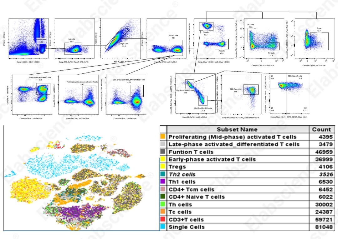
Fig. 1 16-color full-spectral analysis of human peripheral blood T cells and t-SNE dimensionality reduction analysis results.
Table 2. Summary of related flow cytometry antibodies
|
Target |
Clone No. |
Fluorochrome |
Cat. No. |
|
CD8 |
OKT-8 |
Elab Fluor® Violet 610 |
E-AB-F1110T |
|
CCR7/CD197 |
G043H7 |
Elab Fluor® Violet 450 |
E-AB-F1159Q |
|
CD3 |
OKT-3 |
Percp |
E-AB-F1001F |
|
CD4 |
SK3 |
Elab Fluor® 647 |
E-AB-F1352M |
|
CD45RA |
HI100 |
PE/Cyanine7 |
E-AB-F1052H |
|
CD45 |
HI30 |
Elab Fluor® Violet 500 |
E-AB-F1137R |
|
CD28 |
CD28.2 |
APC |
E-AB-F1195E |
|
CD69 |
FN50 |
PE |
E-AB-F1138D |
|
CD45RO |
UCHL1 |
PE/Elab Fluor® 594 |
E-AB-F1139P |
|
CD95 |
DX2 |
Elab Fluor®700 |
E-AB-F1168M1 |
|
CD25 |
BC96 |
PE/Cyanine5 |
E-AB-F1194G |
|
CD127 |
A019D5 |
Elab Fluor® Red 780 |
E-AB-F1152S |
|
CD62L |
DREG56 |
Elab Fluor® Violet 540 |
E-AB-F1051T3 |
|
CD183/CXCR3 |
G025H7 |
FITC |
E-AB-F1156C |
|
CD194/CCR4 |
L291H4 |
PerCP/Cyanine5.5 |
E-AB-F1366J |
|
Live/Dead |
/ |
STYX™ Near-IR |
E-CK-A168 |
03 Best practices for spectral flow cytometry experiments
The following table summarizes several key pitfalls that are most easily overlooked during spectral flow cytometry experiments, along with the corresponding precautions.
Table 3. Spectral flow cytometry experimental considerations and solutions
|
Error-prone steps |
Common pitfalls |
Solutions |
|
Single‑stained controls |
Directly using single‑stained beads instead of single‑stained cells, or ignoring the brightness requirements of single‑stained controls |
Prioritize using single‑stained cells; if beads must be used, at least use a validated protocol with brightness matching |
|
Autofluorescence |
Pursuing "low background" by blindly reducing detector voltage |
Use "complete separation between negative and positive peaks" as the standard for voltage adjustment |
|
Sample clogging |
Ignoring filtration before acquisition, leading to clogged tubing, data loss, or instrument alarms |
Filter the sample using a 40-70 μm mesh; repeat filtration if necessary |
|
Antibody concentration |
Using "more rather than less," relying on the concentration recommended in the datasheet |
Each lot of antibody must be titrated to determine the optimal working concentration |
|
Dye selection |
Packing too many fluorochromes onto a single laser line, increasing the unmixing burden |
Distribute fluorochromes reasonably across laser lines to reduce unmixing pressure at the design stage |
|
Forgetting baseline controls |
Omitting unstained tubes, single‑stained tubes, or experimental controls |
Pre‑list and prepare all necessary controls in the experimental plan |
|
Omitting FMO |
Setting FMO only in conventional panels but ignoring it in high‑parameter experiments |
FMO gating control is a "mandatory configuration" in high‑parameter panels |

